Systems depending on parameters
Download: Jupyter notebook, Julia script, Maple script (PACE called from Maple through UDX, see Using PACE.jl in Maple). To install PACE and run them, see Running the worksheets.
The coefficients of a system often depend on parameters. For each value of the parameters the system has finitely many complex solutions, but the number of real ones changes with the parameters. We describe this for all the values at once:
- the discriminant variety is a hypersurface of the parameter space outside of which the number of real solutions is locally constant: it is constant on each connected component of its complement;
- one sample point in each component, and one exact solving there, give this number everywhere.
This answers the question left open by the worksheet Systems with uncertain coefficients: when does a family of systems keep the real solutions of one instance, and no other?
The discriminant variety factors polynomials: the polynomials are those of Nemo.
using PACE, Nemo

outdir = mktempdir()
struct SVG
    path::String
end
Base.show(io::IO, ::MIME"image/svg+xml", s::SVG) = write(io, read(s.path))
1. One parameter
The unit circle and the horizontal line $y = c$. The variables are $x, y$, the parameter is $c$; all live in the same polynomial ring:
R1, (x, y, c) = polynomial_ring(QQ, ["x", "y", "c"])
line_circle = [x^2 + y^2 - 1, y - c]
discriminant_variety(line_circle, [x, y], [c])
2-element Vector{Vector{Nemo.QQMPolyRingElem}}:
[c - 1]
[c + 1]The discriminant variety is $\{c = -1\} \cup \{c = 1\}$: the line is tangent to the circle. Its complement in $\mathbb{R}$ has three components, $c < -1$, $-1 < c < 1$ and $c > 1$; one sample point in each, and the system solved there:
S, (X, Y) = polynomial_ring(QQ, ["x", "y"])
[(cv, length(real_solutions([X^2 + Y^2 - 1, Y - cv]; prec = 32))) for cv in (-2, 0, 2)]
3-element Vector{Tuple{Int64, Int64}}:
(-2, 0)
(0, 2)
(2, 0)Two real solutions for $-1 < c < 1$, none otherwise. In the worksheet on uncertain coefficients, $c = 1 + 1/1000 \pm 1/100$: this interval contains the point $c = 1$ of the discriminant variety, so that the number of real solutions is not the same for all the systems of the family. This is what the exact instance $c = 1 + 1/1000$ could not see.
2. Two parameters
The family of the worksheet on uncertain coefficients, with its two coefficients now parameters $a$ and $c$:
R, (x, y, a, c) = polynomial_ring(QQ, ["x", "y", "a", "c"])
family = [y^2 - x^3 + a * x, x^2 + y^2 - c]
dv = discriminant_variety(family, [x, y], [a, c])
3-element Vector{Vector{Nemo.QQMPolyRingElem}}:
[a - c]
[c]
[4*a^3 + a^2 + 18*a*c - 27*c^2 + 4*c]Three components: the line $a = c$, the line $c = 0$ and a cubic curve. Together they form a plane curve, whose topology and complement are computed as in the worksheet Topology of a real plane curve. The polynomials are moved to the ring of the parameters, $a$ being the first variable:
P, (pa, pc) = polynomial_ring(QQ, ["a", "c"])
to_params(f) = Nemo.evaluate(f, [zero(P), zero(P), pa, pc])
D = prod(to_params(f) for component in dv for f in component)T = curve_topology(D)
K = curve_complement(T)
curve_summary(T, K)curve: degree 5, 8 terms
critical abscissae: 4 (0 vertical line(s))
(-0.3333333333333333, -0.037037037037037035): critical point, branches left/right = 0/2
(-0.25, 0.0): critical point, branches left/right = 2/2
(0.0, 0.0): critical point, branches left/right = 3/3
(1.0, 1.0): critical point, branches left/right = 2/2
graph: 29 vertices, 36 edges (unbounded branches)
connected components of the curve: 1
complement: 8 connected components (2 bounded, 6 unbounded); Euler check: 8
#1: unbounded, sign +, sample (-2//1, -3//1), 10 boundary arcs in 1 piece(s), neighbours [2, 6]
#2: unbounded, sign -, sample (-2//1, -1//1), 16 boundary arcs in 1 piece(s), neighbours [1, 3, 4]
#3: unbounded, sign +, sample (-2//1, 1//1), 10 boundary arcs in 1 piece(s), neighbours [2, 5, 8]
#4: bounded, sign +, sample (-5//16, -15//512), 8 boundary arcs in 1 piece(s), neighbours [2, 5]
#5: bounded, sign -, sample (-1//8, 1//64), 8 boundary arcs in 1 piece(s), neighbours [3, 4, 7]
#6: unbounded, sign -, sample (1//2, -1//32), 8 boundary arcs in 1 piece(s), neighbours [1, 7]
#7: unbounded, sign +, sample (1//2, 1//4), 8 boundary arcs in 1 piece(s), neighbours [5, 6, 8]
#8: unbounded, sign -, sample (2//1, 33//16), 4 boundary arcs in 1 piece(s), neighbours [3, 7]Eight components. In each, the system is solved at the sample point:
count_at(av, cv) = length(real_solutions([Y^2 - X^3 + av * X, X^2 + Y^2 - cv]; prec = 32))
counts = [(k, comp.sample, count_at(QQ(comp.sample[1]), QQ(comp.sample[2]))) for (k, comp) in enumerate(K)]
8-element Vector{Tuple{Int64, Tuple{Rational{BigInt}, Rational{BigInt}}, Int64}}:
(1, (-2, -3), 0)
(2, (-2, -1), 0)
(3, (-2, 1), 2)
(4, (-5//16, -15//512), 0)
(5, (-1//8, 1//64), 2)
(6, (1//2, -1//32), 0)
(7, (1//2, 1//4), 2)
(8, (2, 33//16), 6)The plane of the parameters, each component in its colour (numbered as above):
SVG(write_curve_svg(joinpath(outdir, "parameters.svg"), T,
                    curve_drawing(T; window = (-3, 3, -3, 4), pixels = (600, 600)), K;
                    title = "discriminant variety in the (a, c) plane"))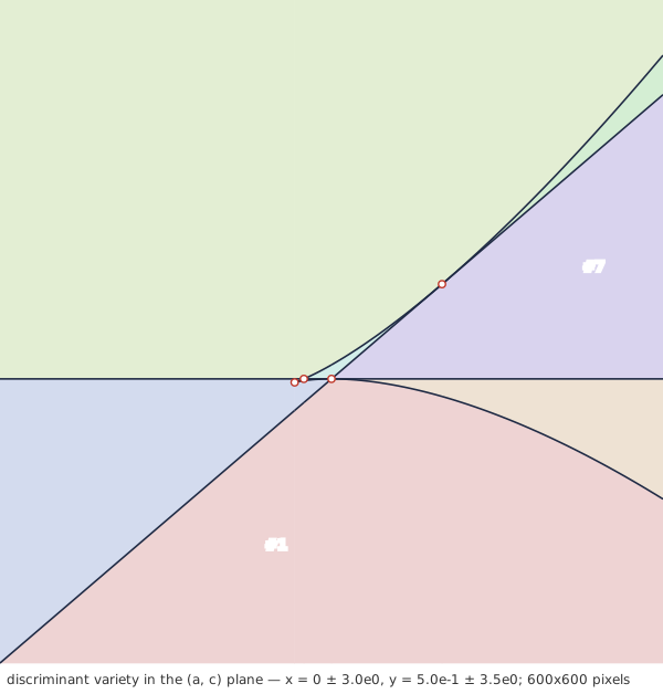
The two bounded components, #4 and #5, are small; around the origin:
SVG(write_curve_svg(joinpath(outdir, "parameters-zoom.svg"), T,
                    curve_drawing(T; window = (-1//2, 1//4, -1//16, 1//16), pixels = (600, 400)), K;
                    title = "around the origin"))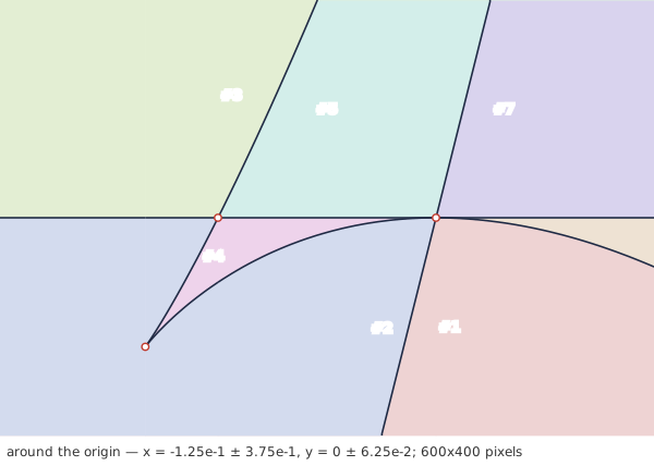
The systems have 0, 2 or 6 real solutions according to the component. The number is the same at every point of a component: the sample point stands for all of them.
3. Back to the uncertain family
The worksheet on uncertain coefficients took $a = 1 \pm e$ and $c = 3 \pm e$. If this box does not meet the discriminant variety, it lies in one component of its complement, and all the systems of the family have the same number of real solutions as the instance $a = 1$, $c = 3$, that is 2.
A sufficient condition: no polynomial of the discriminant variety vanishes on the box, which interval arithmetic proves when the enclosure of its values does not contain $0$. PACE.evaluate takes polynomials of AbstractAlgebra:
import AbstractAlgebra
Q, _ = AbstractAlgebra.polynomial_ring(AbstractAlgebra.QQ, ["a", "c"])
to_aa(f) = Q(Rational{BigInt}.(collect(coefficients(f))), collect(exponent_vectors(f)))
DVQ = [to_aa(to_params(f)) for component in dv for f in component]
3-element Vector{AbstractAlgebra.Generic.MPoly{Rational{BigInt}}}:
a - c
c
4*a^3 + a^2 + 18*a*c - 27*c^2 + 4*cuncertain(q, e) = BigInterval(q; precision = 128) + BigInterval(e; precision = 128) * BigInterval(-1, 1)
meets(e) = [has_zero(z) for z in PACE.evaluate(DVQ, [uncertain(1, e), uncertain(3, e)]; precision = 64)]
[(e, meets(e)) for e in (1//100, 1//10, 1//2, 1)]4-element Vector{Tuple{Real, Vector{Bool}}}:
(1//100, [0, 0, 0])
(1//10, [0, 0, 0])
(1//2, [0, 0, 0])
(1, [1, 0, 1])Up to $e = 1/2$, no component vanishes on the box: every system of the family has exactly two real solutions. With the worksheet on uncertain coefficients, which enclosed the two solutions of every system for $e \le 1/10$, the description is complete: two real solutions, one in each box, and no other.
At $e = 1$ the test fails for $a - c$ and for the cubic. An interval enclosure may contain $0$ without the polynomial vanishing; here the box does meet them: $a = c = 2$ is in it, and the cubic changes sign between two corners:
cubic = only(to_params(f) for component in dv for f in component if total_degree(f) == 3)
[sign(Nemo.evaluate(cubic, [QQ(av), QQ(cv)])) for (av, cv) in ((0, 2), (2, 2))]
2-element Vector{Nemo.QQFieldElem}:
-1
14. More parameters: a partial CAD
With more than two parameters, the components of the complement are no longer given by a curve. partial_CAD gives sample points of the cells of a cylindrical algebraic decomposition adapted to the polynomials of the discriminant variety, in any number of variables; each component of the complement contains at least one cell. Here, in the plane of $(a, c)$:
points = partial_CAD([to_params(f) for component in dv for f in component])
length(points)23[(pt, count_at(QQ(pt[1]), QQ(pt[2]))) for pt in points]23-element Vector{Tuple{Vector{Rational{BigInt}}, Int64}}:
([-7//8, -3//2], 0)
([-7//8, -1//4], 0)
([-7//8, 1//2], 2)
([-9//32, -1], 0)
([-9//32, -1//8], 0)
([-9//32, -1//64], 0)
([-9//32, -1//128], 0)
([-9//32, 1//2], 2)
([-1//8, -5//8], 0)
([-1//8, -1//16], 0)
⋮
([1//2, -1//32], 0)
([1//2, 1//4], 2)
([1//2, 17//32], 2)
([1//2, 1059//1024], 2)
([3//2, -117//128], 0)
([3//2, -1//4], 0)
([3//2, 1], 2)
([3//2, 97//64], 6)
([3//2, 1065//512], 2)23 cells for 8 components: the decomposition cuts the plane by vertical lines, and several cells lie in the same component. The numbers of real solutions found are again 0, 2 and 6.
5. Square systems: the discriminant variety from LACE
discriminant_variety handles any system that is generically zero-dimensional in the unknowns, and splits its result into irreducible components (with DiscriminantVariety.jl). When the system has as many equations as unknowns, the discriminant variety is the union of two sets that the C library of LACE computes directly:
\[W_c\]
, the critical values: the projection on the parameters of the solutions where the Jacobian determinant with respect to the unknowns vanishes, that is the elimination ideal of the system augmented by this determinant (eliminate);\[W_\infty\]
, the parameters where solutions go to infinity (ideals_at_infinity).
No factorization is needed. For the family of section 2:
jacobian_det(F, vars) = det(matrix(parent(F[1]), [derivative(f, v) for f in F, v in vars]))
Wc = eliminate(vcat(family, [jacobian_det(family, [x, y])]), [x, y])
1-element Vector{Nemo.QQMPolyRingElem}:
4*a^4*c - 4*a^3*c^2 + a^3*c + 17*a^2*c^2 - 45*a*c^3 + 4*a*c^2 + 27*c^4 - 4*c^3ideals_at_infinity(family, [x, y])(true, Vector{Nemo.QQMPolyRingElem}[[1], [1]])\[W_c\]
is the polynomial $D$ of section 2, the product of the three components, and $W_\infty$ is empty ([1] for each unknown): no solution goes to infinity.
Solutions at infinity
For $a x^2 + y^2 = 1$ and $x = y$, that is $(a + 1)x^2 = 1$:
R5, (x5, y5, a5) = polynomial_ring(QQ, ["x", "y", "a"])
F5 = [a5 * x5^2 + y5^2 - 1, x5 - y5]
eliminate(vcat(F5, [jacobian_det(F5, [x5, y5])]), [x5, y5]), ideals_at_infinity(F5, [x5, y5])
(Nemo.QQMPolyRingElem[1], (true, Vector{Nemo.QQMPolyRingElem}[[1], [a + 1]]))\[W_c\]
is empty: the solutions are never double. But at $a = -1$ the two solutions $\pm 1/\sqrt{a+1}$ go to infinity, and $W_\infty$ gives $a + 1$. On each side:
[(av, length(real_solutions([av * X^2 + Y^2 - 1, X - Y]; prec = 32))) for av in (-2, 0)]2-element Vector{Tuple{Int64, Int64}}:
(-2, 0)
(0, 2)A larger system
Three equations in three unknowns $u, v, w$, two parameters $p, q$:
R6, (u, v, w, p, q) = polynomial_ring(QQ, ["u", "v", "w", "p", "q"])
F6 = [u^2 + p * v^2 + w - 1, v^2 - q * u * w + u - 2, w^2 + u * v + p * q * w - 3]
t_lace = @elapsed begin
    Wc6 = eliminate(vcat(F6, [jacobian_det(F6, [u, v, w])]), [u, v, w])
    zerodim6, Winf6 = ideals_at_infinity(F6, [u, v, w])
end
[total_degree(f) for f in Wc6], Winf6, t_lace
([45], Vector{Nemo.QQMPolyRingElem}[[1], [1], [p^3*q^4 + 1]], 1.069225997)\[W_c\]
is a curve of degree 45, and solutions go to infinity on $p^3q^4 + 1 = 0$. The same discriminant variety with DiscriminantVariety.jl alone (dv_backend!(:julia)), after a first call on the small system above, so that its compilation is not counted:
dv_backend!(:julia)
discriminant_variety(F5, [x5, y5], [a5])
t_dv = @elapsed discriminant_variety(F6, [u, v, w], [p, q])
dv_backend!(:lace)
t_lace, t_dv
(1.069225997, 3.927643735)The regions of the $(p, q)$ plane, and the number of real solutions in each:
P6, (pp, pq) = polynomial_ring(QQ, ["p", "q"])
to_pq(f) = Nemo.evaluate(f, [zero(P6), zero(P6), zero(P6), pp, pq])
D6 = prod(to_pq(f) for f in vcat(Wc6, Winf6...) if !isone(f))
T6 = curve_topology(D6)
K6 = curve_complement(T6)
length(K6)42S6, (U, V, W) = polynomial_ring(QQ, ["u", "v", "w"])
function count6(pv, qv)
sys = [U^2 + pv * V^2 + W - 1, V^2 - qv * U * W + U - 2, W^2 + U * V + pv * qv * W - 3]
return length(real_solutions(sys; prec = 32))
end
counts6 = [count6(QQ(k.sample[1]), QQ(k.sample[2])) for k in K6]
[(n, count(==(n), counts6)) for n in sort(unique(counts6))]5-element Vector{Tuple{Int64, Int64}}:
(0, 1)
(2, 5)
(4, 16)
(6, 17)
(8, 3)42 regions, with 0 to 8 real solutions. They spread from $p \approx -150$ to $|q| \approx 10^9$; the window $[-6, 2] \times [-2, 2]$ of the $(p, q)$ plane:
SVG(write_curve_svg(joinpath(outdir, "pq.svg"), T6,
                    curve_drawing(T6; window = (-6, 2, -2, 2), pixels = (600, 600)), K6;
                    title = "discriminant variety in the (p, q) plane"))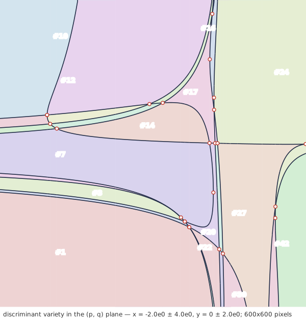
All of them, up to a homeomorphism of the plane:
SVG(write_curve_svg_topo(joinpath(outdir, "pq-topo.svg"), T6, K6))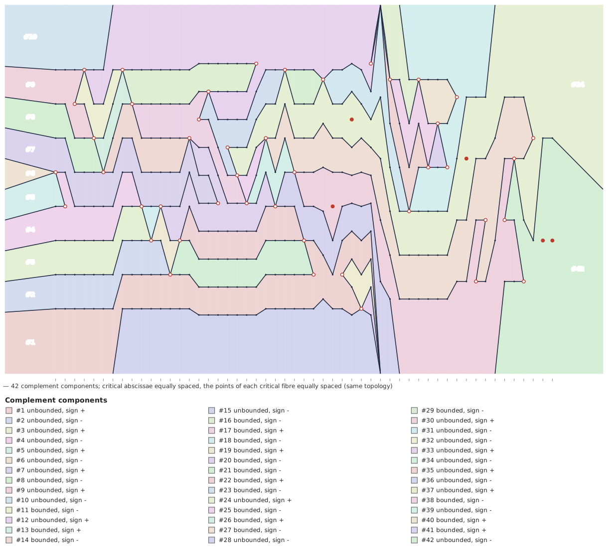
6. A constraint $g \neq 0$: a discriminant variety by hand
The system of section 2, with its second equation multiplied by $x$, and the constraint $x \neq 0$:
R7, (x, y, a, c) = polynomial_ring(QQ, ["x", "y", "a", "c"])
F7 = [y^2 - x^3 + a * x, x * (x^2 + y^2 - c)]
2-element Vector{Nemo.QQMPolyRingElem}:
-x^3 + x*a + y^2
x^3 + x*y^2 - x*cThe point $(0, 0)$ is a solution for every value of the parameters, and the Jacobian determinant vanishes there: the critical values fill the whole plane, and the elimination ideal is the zero ideal.
J7 = jacobian_det(F7, [x, y])
eliminate(vcat(F7, [J7]), [x, y])Nemo.QQMPolyRingElem[]The constraint removes this solution. saturate(F, g, vars) computes $(\langle F \rangle : g^\infty) \cap \mathbb{Q}[\text{params}]$, the elimination ideal without the solutions where $g$ vanishes; with no variable to eliminate, it gives the saturated system itself, whose solutions are those of $F$ with $x \neq 0$:
S7 = saturate(F7, x, elem_type(R7)[])3-element Vector{Nemo.QQMPolyRingElem}:
x^2 + y^2 - c
x*y^2 + x*a - x*c + y^2
x*a - x*c + y^4 + y^2*a - 2*y^2*c + y^2 - a*c + c^2The discriminant variety of the system under the constraint is assembled from three parts, each computed by LACE:
\[W_c\]
, the critical values, away from $x = 0$;\[W_g\]
, the parameters where a solution reaches $x = 0$: the elimination ideal of the saturated system augmented by $x$;\[W_\infty\]
, the parameters where solutions go to infinity.
Wc7 = saturate(vcat(F7, [J7]), x, [x, y])1-element Vector{Nemo.QQMPolyRingElem}:
4*a^4 - 4*a^3*c + a^3 + 17*a^2*c - 45*a*c^2 + 4*a*c + 27*c^3 - 4*c^2Wg7 = eliminate(vcat(S7, [x]), [x, y])1-element Vector{Nemo.QQMPolyRingElem}:
cideals_at_infinity(F7, [x, y])(true, Vector{Nemo.QQMPolyRingElem}[[1], [1]])\[W_c\]
is $(a - c)$ times the cubic of section 2, $W_g$ is the line $c = 0$, and no solution goes to infinity. Their union is the curve $D$ of section 2:
D7 = prod(to_params(f) for f in vcat(Wc7, Wg7) if !isone(f))
D7 == DtrueAs expected: with $x \neq 0$, the system is the one of section 2. In each component of the complement, the solutions with $x \neq 0$ are those of the saturated system; the system itself has one more, the point $(0, 0)$:
at(f, av, cv) = Nemo.evaluate(f, [X, Y, S(av), S(cv)])
function counts7(av, cv)
    with_constraint = length(real_solutions([at(f, av, cv) for f in S7]; prec = 32))
    all_solutions = length(real_solutions([at(f, av, cv) for f in F7]; prec = 32))
    return (x_nonzero = with_constraint, all = all_solutions)
end
[(k, counts7(QQ(comp.sample[1]), QQ(comp.sample[2]))...) for (k, comp) in enumerate(K)]
8-element Vector{Tuple{Int64, Int64, Int64}}:
(1, 0, 1)
(2, 0, 1)
(3, 2, 3)
(4, 0, 1)
(5, 2, 3)
(6, 0, 1)
(7, 2, 3)
(8, 6, 7)