The H∞ norm: sampling, exact peak gain, and the curve behind it

Download: Jupyter notebook, Julia script, Maple version (same conclusions). To install PACE and run them, see Running the worksheets.

A stable linear system with transfer matrix $G(s)$ answers an input at frequency $\omega$ with an amplification given by the matrix $G(i\omega)$. For a system with one input and one output, this amplification is the number $|G(i\omega)|$; with several inputs and outputs, it is the largest singular value $\sigma_{\max}(G(i\omega))$, the largest factor by which $G(i\omega)$ multiplies the length of a vector. The $H_\infty$ norm is the largest amplification over all frequencies, the peak gain: $\gamma = \sup_{\omega\in\mathbb{R}} \sigma_{\max}\bigl(G(i\omega)\bigr).$

Numerically, $\gamma$ is estimated by computing the amplification at a list of frequencies, or computed by the bisection method of Boyd, Balakrishnan and Kabamba and its variants (Matlab's hinfnorm and getPeakGain), which need a tolerance. Exactly, $\gamma^2$ is the largest critical value of a plane algebraic curve (section 4), and it can be enclosed between two rationals.

Two certified implementations of PaceControl, both built on LACE, are used: hinf_peak, which encloses $\gamma^2$, and Hinf_StHa, which encloses $\gamma$ with Sturm-Habicht sequences (signed subresultants).

using LinearAlgebra, Nemo, PaceControl, PACE
using PaceControl: HinfNorm
import AbstractAlgebra

1. A sharp resonance

A lightly damped oscillator, with one input and one output: $G(s) = 1/(s^2 + 2\zeta s + 1)$ with damping $\zeta = 10^{-3}$. Near $\omega = 1$ the amplification has a very narrow and high peak. Its value is known in closed form: $\gamma = 1/(2\zeta\sqrt{1-\zeta^2}) \approx 500.00025$, at $\omega = \sqrt{1-2\zeta^2}$.

ζ = 1 // 1000
γ_exact = 1 / (2 * Float64(ζ) * sqrt(1 - Float64(ζ)^2))

500.0002500001875

Sampling 200 frequencies, logarithmically spaced over four decades, as a Bode plot would:

G(ω) = 1 / ((im * ω)^2 + 2 * Float64(ζ) * im * ω + 1)
ωs = 10 .^ range(-2, 2, length = 200)
maximum(abs.(G.(ωs)))

22.089396762022933

The resonance is narrower than the spacing of the grid: the estimate is more than 20 times too small, and nothing in the result says so.

hinf_peak takes the numerator and the denominator of $G$ by their coefficients, constant term first, and encloses $\gamma^2$ between two rationals:

r = hinf_peak([1], [1, 2ζ, 1])
(Float64(r.lo), Float64(r.hi), r.lo <= 1 / (4ζ^2 * (1 - ζ^2)) <= r.hi)

(250000.25000025, 250000.25000025, true)

The Sturm-Habicht method, on the transfer function itself, encloses $\gamma$:

S1, (y, s) = AbstractAlgebra.rational_function_field(AbstractAlgebra.QQ, [:y, :s])
Hinf_StHa([1 // (s^2 + 2ζ * s + 1);;]; starting_precision = Int32(60))

[500.0002500001875001562501367187404348327, 500.0002500001875001562501367190094744039]

Two independent certified methods, and the closed form, agree.

2. A pole on the imaginary axis

With $\zeta = 0$ there is no damping: $G = 1/(s^2+1)$ has poles at $\pm i$, the amplification is infinite at $\omega = 1$, and so is $\gamma$. A sampling returns a finite number, large or not depending on how close a sample falls to $\omega = 1$:

G0(ω) = 1 / (1 - ω^2)
maximum(abs.(G0.(ωs)))

22.110007263447283

The exact method decides that a root of the denominator lies on the axis:

hinf_peak([1], [1, 0, 1]).infinite

true

3. A model from COMPleib: AC1

COMPleib (Leibfritz, 2004) is a library of benchmark models for control design. AC1 is an aircraft model: $\dot x = Ax + B_1w$, $z = C_1x + D_{11}w$, with $5$ states, $3$ inputs $w$ and $2$ outputs $z$, so that $G(s) = C_1(sI-A)^{-1}B_1 + D_{11}$ is a $2\times3$ matrix. Its data are decimal numbers, read as the rationals they spell ($0.1$ as $1/10$).

M = read_matrices(joinpath(pkgdir(PaceControl), "test", "data", "AC1_matrices.txt"))
A, B, C, Dm = (Float64.(M[k]) for k in ("A", "B1", "C1", "D11"))
size(A), size(B), size(C)

((5, 5), (5, 3), (2, 5))

Sampling $\sigma_{\max}(G(i\omega))$:

σmax(ω) = opnorm(C * ((im * ω * I - A) \ B) + Dm)
maximum(σmax.(ωs))

2.155675190547939

Here the sampling is close, $0.6\,\%$ below the true value, but only a certified computation tells how close. The exact peak gain, with the frequency where it is attained:

r = hinf_peak(M)
(γ² = (Float64(r.lo), Float64(r.hi)), ω² = (Float64(r.olo), Float64(r.ohi)), where = r.src)

(γ² = (4.706053414358383, 4.706053414358383), ω² = (0.03336274011557644, 0.03336274011557644), where = :critique)

The peak is attained at a finite, nonzero frequency (where = :critique: a critical point of the curve of section 4), and $\gamma \approx$

sqrt(Float64(r.lo))

2.169344005536785

4. The curve behind the norm

The squared singular values $\Gamma$ of $G(i\omega)$, as functions of $\Omega=\omega^2$, lie on the real algebraic curve $c(\Gamma,\Omega) = 0$, the numerator of $\det(\Gamma I - G^T(-s)G(s))$ with $s^2=-\Omega$. Its degrees in $\Gamma$ and $\Omega$:

cr = HinfNorm.curve(HinfNorm.shared_parts(M))
(cr.degG, cr.degO)

(2, 4)

Its coefficients are exact integers; the largest has this many digits:

maximum(ndigits.(collect(coefficients(cr.c))))

93

\[\gamma^2\]

is the largest critical value of $\Gamma$ on the branch $\Omega\ge0$ (or a limit at $\Omega = 0$ or $\infty$). CurveTopology computes the certified topology of the curve and draws it, here with $\Omega$ horizontal and $\Gamma$ vertical, around the peak:

R2, (x, y) = polynomial_ring(ZZ, ["x", "y"])
c = Nemo.evaluate(cr.c, [y, x])            ## x = Ω, y = Γ
T = curve_topology(c)
Dr = curve_drawing(T; window = (0.0, 4 * Float64(r.olo), 0.0, 1.4 * Float64(r.lo)))
write_curve_svg("ac1_curve.svg", T, Dr; title = "AC1: squared singular values Γ against Ω = ω²");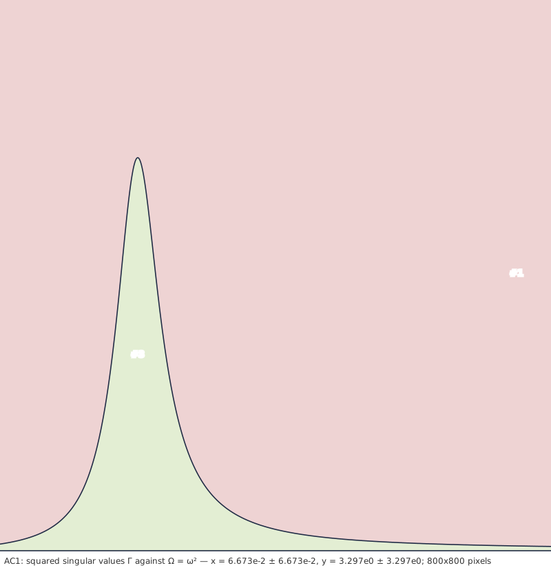

The top of the branch is the certified $(\Omega, \Gamma) \approx (0.0334, 4.706)$.

5. The Sturm-Habicht method

Hinf_StHa follows Bouzidi, Quadrat, Rouillier and Younes (2021). Let us denote by $RL_\infty$ the algebra of real rational functions on the imaginary axis $i\mathbb{R}$ which are proper and have no pole on $i\mathbb{R}$. For a transfer matrix $G \in \mathbb{R}(s)^{u\times v}$ whose entries, on $i\mathbb{R}$, are in $RL_\infty$, and for $\gamma > 0$, let

\[\Phi_\gamma(s) = \gamma^2 I_v - G^T(-s)\,G(s).\]

One can write $\det \Phi_\gamma(i\omega) = n(\omega,\gamma)/d(\omega)$ with $n$ and $d$ coprime, and $d$ does not vanish on $\mathbb{R}$ since $G$ has no pole on the imaginary axis. Let $\tilde n$ be the square-free part of $n$ and $L_\omega(\tilde n)$ its leading coefficient in $\omega$. Then

\[\|G\|_\infty = \max\Bigl(\pi_\gamma\bigl(V_\mathbb{R}(\tilde n, \partial\tilde n/\partial\omega)\bigr) \cup V_\mathbb{R}\bigl(L_\omega(\tilde n)\bigr)\Bigr),\]

where $V_\mathbb{R}$ denotes the real zeros and $\pi_\gamma$ the projection on the $\gamma$ axis: the norm is a critical value of the curve $\tilde n = 0$, or a value of $\gamma$ where a branch goes to infinity.

The algorithm takes a polynomial $P \in \mathbb{Z}[\gamma][\omega]$ whose real curve is bounded in the $\gamma$ direction, and returns an isolating interval of this maximum:

1. compute the signed subresultant (Sturm-Habicht) sequence of $P$ and $\partial P/\partial\omega$ with respect to $\omega$;
2. isolate the real roots $\gamma_1 < \dots < \gamma_m$ of its last element $\mathrm{Sres}_0$;
3. scan them from $\gamma_m$ downwards, and return the first one which is a root of the leading coefficient of $P$, or at which the principal Sturm-Habicht coefficients $\mathrm{stha}_d, \dots, \mathrm{stha}_1$ have at least one sign variation.

Hinf_StHa takes either the transfer matrix or the polynomial $n$. With a transfer matrix over $\mathbb{Q}(s)$:

S2, (y2, s2) = AbstractAlgebra.rational_function_field(AbstractAlgebra.QQ, [:y, :s])
G2 = [s2 // (s2 + 1) -s2 // (s2 + 1); -s2 // (s2 + 1) 1 // (s2 + 1)]
Hinf_StHa(G2)

[1.53125, 1.765625]

The result is an interval at the precision starting_precision, in bits, or finer:

Hinf_StHa(G2; starting_precision = Int32(10))

[1.618033988749894848204586834364286749966, 1.618033988749894848204586834367002543677]

With the polynomial $n(\omega,\gamma)$, as a polynomial in $\omega$ with coefficients in $\mathbb{Q}[\gamma]$:

Sγ, γ = polynomial_ring(Nemo.QQ, "γ")
Sω, ω = polynomial_ring(Sγ, "ω")
P = (4γ - 1) * (4γ + 1) * ω^4 - 4 * (2γ - 1) * (2γ + 1) * ω^2 + 16 * (γ - 1) * (γ + 1)
Hinf_StHa(P)

[1.09375, 1.125]

Hinf_StHa(P; starting_precision = Int32(10))

[1.094450529658366971007265523781985827874, 1.094450529658366971007265523790531412044]

Summary

The norm is a critical value of an algebraic curve: certified real solving decides which candidate is the maximum, and the topology of the curve shows it.

References

• S. Boyd, V. Balakrishnan, P. Kabamba, A bisection method for computing the $H_\infty$ norm of a transfer matrix and related problems, Mathematics of Control, Signals and Systems 2(3), 207-219, 1989.
• M. Kanno, M. C. Smith, Validated numerical computation of the $\mathcal{L}_\infty$-norm for linear dynamical systems, Journal of Symbolic Computation 41(6), 697-707, 2006.
• Y. Bouzidi, A. Quadrat, F. Rouillier, G. Younes, Computation of the $\mathcal{L}_\infty$-norm of finite-dimensional linear systems, in Maple in Mathematics Education and Research, Springer, 119-136, 2021, doi:10.1007/978-3-030-81698-8_9.
• A. Quadrat, F. Rouillier, G. Younes, $\ell_\infty$-norm computation for linear time-invariant systems depending on parameters, Maple Transactions 4(1), 2024, doi:10.5206/mt.v4i1.17129.
• F. Leibfritz, COMPleib: COnstrained Matrix-optimization Problem library, University of Trier, 2004.