Stability regions in a parameter plane
Download: Jupyter notebook, Julia script, Maple version (same conclusions). To install PACE and run them, see Running the worksheets.
A multidimensional discrete linear system with rational transfer function $G = N/D$ is structurally stable when its denominator $D$ has no zero in the closed unit polydisc $\overline{\mathbb{U}}^n = \{z \in \mathbb{C}^n \mid |z_1| \le 1, \dots, |z_n| \le 1\}$. By a theorem of DeCarlo, Murray and Saeks (1977), this holds if and only if
- each univariate polynomial $D(1, \dots, 1, z_k, 1, \dots, 1)$ has no root in $|z_k| \le 1$, for $k = 1, \dots, n$;
\[D\]
has no zero on the torus $|z_1| = \dots = |z_n| = 1$.
The first conditions are Hurwitz tests after the change of variable $z = (1-x)/(1+x)$, decided by signed subresultant (Sturm-Habicht) sequences. For the second one, the Möbius map $z_k = (x_k - i)/(x_k + i)$ turns the torus into $\mathbb{R}^n$, and the condition becomes: the system $\{\mathcal{R} = 0, \mathcal{I} = 0\}$, where $\mathcal{R}$ and $\mathcal{I}$ are the real and imaginary parts of the numerator of $D$, has no real solution. The case $n = 2$ without parameters is treated in the 2-D stability worksheet.
When the denominator $D(z_1,z_2,u_1,u_2)$ of a 2-D system depends on two parameters, the question becomes: for which $(u_1,u_2)$ is the system structurally stable? The answer is a union of regions of the parameter plane, bounded by algebraic curves. We compute these curves exactly, take one rational point in each region, and decide stability there with the non-parametric test of the 2-D stability worksheet.
Example from the literature (Li, Hou, 2021): $D = u_2 z_1 z_2 - u_1 z_2 - u_2 z_1 + z_1 z_2 - z_1 + 1 .$
stability_parametric takes $D$ in a ring over ComplexField (the Möbius map introduces $i$); its coefficients must be integers, which are exact there.
using Nemo, PACE, PaceControl

Rc, (z1, z2, u1, u2) = polynomial_ring(Nemo.ComplexField(), ["z1", "z2", "u1", "u2"])
D = u2 * z1 * z2 - u1 * z2 - u2 * z1 + z1 * z2 - z1 + 11. The polynomial conditions
As in the 2-D stability worksheet, with the parameters kept symbolic: $\mathcal{R}$ and $\mathcal{I}$ (the torus, after the Möbius map), and $D_1$, $D_2$ (the two discs, after $z = (1-x)/(1+x)$, to be Hurwitz).
RD, CD, D1, D2 = PaceControl.prepare_input_stability(D)(-x*y*u1 + x*y - u1 - 2*u2 - 3, x*u1 - 2*x*u2 - x - y*u1 + y, (-u1 + 1)*x - u1 + 1, (u1 - 2*u2 - 1)*x - u1 + 1)2. Where can the answer change?
On the torus. The number of real solutions of $\{\mathcal{R}=\mathcal{I}=0\}$ is locally constant outside the discriminant variety of the system with respect to $(u_1,u_2)$ (LACE, DiscriminantVariety):
R = parent(RD)
dv = discriminant_variety([RD, CD], gens(R)[1:2], gens(R)[3:4])
3-element Vector{Vector{Nemo.QQMPolyRingElem}}:
[u1 + 2*u2 + 3]
[u1 - 2*u2 - 1]
[u1 - 1]On the discs. The parametric Liénard-Chipart criterion gives polynomials in $u$ whose signs decide whether $D_1$ and $D_2$ are Hurwitz: for each of them, its coefficients and the signed principal subresultant coefficients of its even and odd parts, all nonzero and of the sign of its leading coefficient:
lc1, sr1 = lienard_chipart(D1)
lc2, sr2 = lienard_chipart(D2)
lcs = vcat(lc1, sr1, lc2, sr2)
8-element Vector{Nemo.QQMPolyRingElem}:
-u1 + 1
-u1 + 1
-u1 + 1
-u1 + 1
-u1 + 1
u1 - 2*u2 - 1
u1 - 2*u2 - 1
-u1 + 1The boundary of the regions is contained in the zero set of the irreducible factors of all these polynomials:
Ru, (a, b) = polynomial_ring(QQ, ["u1", "u2"])
to_u(p) = Ru(collect(coefficients(p)), map(v -> v[end-1:end], collect(exponent_vectors(p))))
polys = unique(filter(p -> !is_constant(p), vcat(to_u.(vcat(dv...)), to_u.(lcs))))
boundary = unique(vcat([first.(collect(factor(p))) for p in polys]...))
3-element Vector{Nemo.QQMPolyRingElem}:
u1 + 2*u2 + 3
u1 - 2*u2 - 1
u1 - 1Three lines.
3. One point per region
Partial CAD. A cylindrical decomposition of the plane adapted to these curves gives one rational point in each cell of maximal dimension; stability_parametric runs the non-parametric test at each of them:
stable, unstable = stability_parametric(D)
(length(stable), length(unstable))
(1, 11)stable1-element Vector{Any}:
Rational{BigInt}[0, -1]Connected components. A CAD cuts the regions into cylindrical cells, more than needed. The certified topology of the curve $\prod q = 0$ (CurveTopology) gives the connected components of its complement, each with a rational sample point:
T = curve_topology(prod(boundary))
K = curve_complement(T)
[k.sample for k in K]
7-element Vector{Tuple{Rational{BigInt}, Rational{BigInt}}}:
(-2, -3)
(-2, -1)
(-2, 1)
(0, -1)
(2, -9)
(2, -2)
(2, 5)The test at a sample point: the Liénard-Chipart signs, then the real solutions of $\{\mathcal{R}=\mathcal{I}=0\}$ with the parameters replaced by their values (the bivariate solver of LACE, as in the 2-D stability worksheet):
The bivariate RUR of LACE (no Gröbner basis), then the certified real solutions. A constant resultant means no solution, reported as a PACEError of code -1.
function biv_real_solutions(a, b)
    comps = try
        biv_parameterization([a, b]; verbose = false)
    catch e
        e isa PACEError && e.code == -1 || rethrow()
        []
    end
    vcat([real_solutions(c.rext, c.rden, [c.num_Y, c.num_X]; prec = 30) for c in comps]...)
end

Rxy, (x, y) = polynomial_ring(QQ, ["x", "y"])

function hurwitz_at(coefs, sres, p)
    s = sign(coefs[end](p...))      ## leading coefficient
    s != 0 && all(f -> sign(f(p...)) == s, vcat(coefs, sres))
end

function stable_at(p)
    hurwitz_at(lc1, sr1, p) && hurwitz_at(lc2, sr2, p) || return false
    a, b = (Nemo.evaluate(f, [x, y, Rxy(p[1]), Rxy(p[2])]) for f in (RD, CD))
    isempty(biv_real_solutions(a, b))
end

verdict = [stable_at(k.sample) for k in K]
7-element Vector{Bool}:
0
0
0
1
0
0
0Seven regions, twelve CAD cells; one stable region in both cases.
4. The stable region
Its description by signs of the boundary polynomials:
p = K[findfirst(verdict)].sample
[(q, sign(q(p...))) for q in boundary]
3-element Vector{Tuple{Nemo.QQMPolyRingElem, Nemo.QQFieldElem}}:
(u1 + 2*u2 + 3, 1)
(u1 - 2*u2 - 1, 1)
(u1 - 1, -1)The system is stable exactly in the open triangle $u_1 < 1,\ u_1 - 2u_2 > 1,\ u_1 + 2u_2 > -3$, of vertices $(1,0)$, $(1,-2)$, $(-1,-1)$. The drawing, each region in its colour (the stable one contains $(0,-1)$):
Dr = curve_drawing(T; window = (-4.0, 3.0, -4.0, 3.0))
write_curve_svg("stability_regions.svg", T, Dr, K; title = "Regions of the (u1, u2) plane");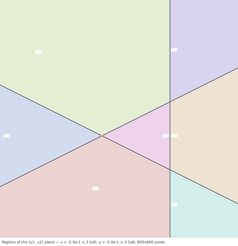
Summary
| Step | Tool |
|---|---|
| conditions on the torus and on the discs | Möbius maps, exact (PaceControl) |
| where the number of real solutions can change | discriminant variety (LACE, DiscriminantVariety) |
| where the Hurwitz conditions can change | parametric Liénard-Chipart (PACE) |
| one point per region | partial CAD (PACE), or the complement of the curve (CurveTopology) |
| the answer in each region | RUR and certified isolation (LACE) |
The result is exact: a finite list of regions, each certified stable or unstable. A grid of the parameter plane would only give a picture, blind to regions smaller than its step.
References
- R. A. DeCarlo, J. Murray, R. Saeks, Multivariable Nyquist theory, International Journal of Control 25(5), 657-675, 1977.
- D. Lazard, F. Rouillier, Solving parametric polynomial systems, Journal of Symbolic Computation 42(6), 636-667, 2007.
- Y. Bouzidi, F. Rouillier, Certified algorithms for proving the structural stability of two dimensional systems possibly with parameters, MTNS 2016, 41-48.
- Y. Bouzidi, A. Quadrat, F. Rouillier, Certified non-conservative tests for the structural stability of discrete multidimensional systems, Multidimensional Systems and Signal Processing 30(3), 1205-1235, 2019.
- X. Li, X. Hou, A new approach based on the discriminant system of polynomial for robust stability and stabilization of two-dimensional systems, Journal of the Franklin Institute 358(5), 2597-2622, 2021.